Diffusion

GRAPHS

% This code simulates a diffusion equation on a 1D spatial domain [-L,L];
% It is a {\bf Fickian} diffusion
% A reaction term F(u) can be added. For instance F(u)=ru(1-u/K).
% Determine a function u(t,x) as a matrix where lines correspond to
% different time steps and columns correspond to different space locations.

% Initial Conditions are provided in the variable CI and plotted on
% Figure(1)
% Boundary conditions are Dirichlet conditions at infinity (u->0 when
% x->+/-\infty
% The diffusion coefficient is space dependent and given in function
% DiffCoef.m, its derivative is needed and given in dDiffCoef.m

% Jean-Christophe POGGIALE - Mars 2016

clear all;clc;
global A B M L p reac

%Parameter setting
A=0.2;B=0.2; % Define the diffusion coefficient

tmax=20; % Time length of the simulation
dt=0.1; % Time step
dx=0.05; % Space step
L=10;     % Domain=[-L,L]
x=-L:dx:L; % Define the space mesh
r=2;K=2;p=[r;K]; % Parameters of the reaction term, inserted in a vector p

% OPTIONS %%%%%%%%%%%%%%%%%%%%%%%%%%%%%%%%%%%%%%%%%%%%%%%%%%%%%%%%%%%%%
BC0flux=0; % if =1 then no flux at the boundaries -L and L, else L and -L are not boundaries
reac=0;     % if =1 then the reaction term is included in the simulation
SolAnalyt=1; % if =1, compares the numerical solution to the analytical solution
%%%%%%%%%%%%%%%%%%%%%%%%%%%%%%%%%%%%%%%%%%%%%%%%%%%%%%%%%%%%%%%%%%%%%%%

% Initial conditions
x0=0;% Center of the initial distribution
sigma=0.1;
CI=exp(-((x-x0)/sigma).^2); % Gaussian curve around x_0
CI=CI/(sum(CI)*dx); % Normalization, the total amount of matter is 1

% Calculus of the diffusion matrix
D=DiffCoef(x);
dD=dDiffCoef(x);
M=diag(-2*D/dx^2);
MU=diag((dD(1:end-1)/2+D(1:end-1)/dx)/dx,1);
ML=diag((D(2:end)/dx-dD(2:end)/2)/dx,-1);
M=M+ML+MU;

% Neuman Boundary conditions for a closed domain
if BC0flux==1
    M(1,2)=2*D(1,2)/dx^2;
    M(end,end-1)=2*D(end,end-1)/dx^2;
end



% Running simulation
[t u]=ode45(@ModelDiff1D,0:dt:tmax,CI);

% Analytical Solution
t0=sigma^2/(2*DiffCoef(x0));
i=1;UA=[];
for i=0:length(t)
    uA=GaussFunct(t0+i*dt,x,x0,DiffCoef(x0),t0);
    UA=[UA;uA];
end

GRAPHS

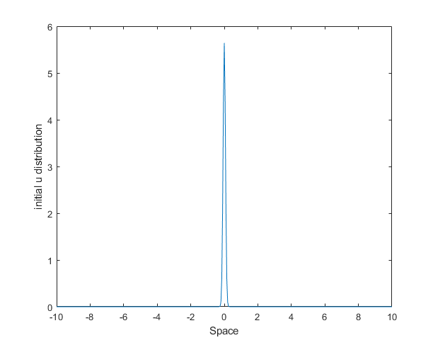
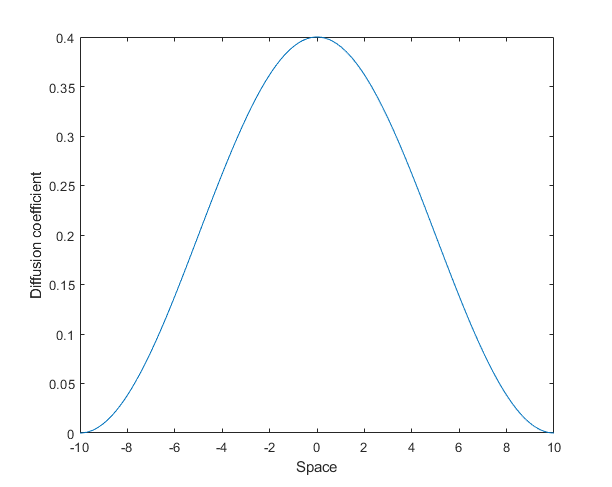
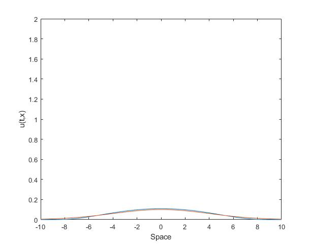
figure(1) % Initial Condition
plot(x,CI)
xlabel('Space');ylabel('initial u distribution');

figure(2) % Diffusion coefficient as a function of space
plot(x,D);
ylim([0 max(D)])
xlabel('Space');ylabel('Diffusion coefficient');

figure(3) % dynamics of u on the spatial domaine
for i=1:length(t)
    if SolAnalyt==1
        plot(x,u(i,:),x,UA(i,:));
    else
        plot(x,u(i,:));
    end
    xlim([-L L]);
    ylim([0 2])
    xlabel('Space');ylabel('u(t,x)')
    F(i)=getframe;
end

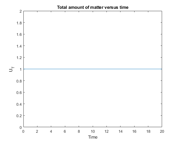
figure(4) % Total amount of matter versus time
S=sum(u')*dx;S=S';
plot(t,S)
ylim([0 max(S)+1])
xlabel('Time');ylabel('U_T');
title('Total amount of matter versus time')

Contents

GRAPHS