% Code de simulation et d'analyse du modèle de Ronsenzweig-McArthur
% J.-C. Poggiale - Mai 2015

clear all; clc;
global r K a b e m
r=1;K=1.53;a=1;b=1;e=0.5;m=0.1;
K=1.4;K00=K;
tmax=200;dt=0.1;
x0=1;y0=1;

nbx=100; % Nombre de points sur l'isocline des proies

CI=[x0,y0];duree=0:dt:tmax;


xe=m/(e*a-m*b);
ye=isoclineprey(xe);

[t u]=ode45(@RMA,duree,CI);
x=u(:,1);y=u(:,2);

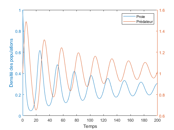
figure(1)
plotyy(t,x,t,y)
xlabel('Temps');ylabel('Densité des populations');
legend('Proie','Prédateur')

dx=K/nbx;xx=0:dx:K;
yy=isoclineprey(xx);
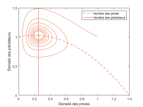
figure(2)
plot(xx,yy,'r--')
xlabel('Densité des proies');ylabel('Densité des prédateurs');
hold on
line([xe xe],[0 max(y)],'Color',[1,0,0])
plot(x,y,xe,ye,'go')
legend('Isocline des proies','Isocline des prédateurs')
hold off


Kmin=0.1;Kmax=3;dK=0.1;
Kmin=xe;Ue=[];
Lambda=[];YE=[];YEnum=[];uenum=[xe ye];
J11=[];J12=[];J21=[];J22=[];Ktamp=K;
for K=Kmin:dK:Kmax
    ye=isoclineprey(xe);
    ue=[xe ye];YE=[YE;ye];
    Ue=[Ue;ue];
    uenum=fsolve(@RMA2,uenum);YEnum=[YEnum;uenum];
    J=JacobMat(ue);
    J11=[J11 J(1,1)];J12=[J12 J(1,2)];J21=[J21 J(2,1)];J22=[J22 J(2,2)];
    Lambda=[Lambda;max(real(eig(J)))];
    %Lambda=[Lambda real(eig(J))];
end
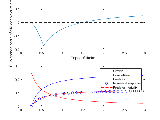
figure(3)
subplot(2,1,1)
KK=Kmin:dK:Kmax;
plot(KK,Lambda,[0 Kmax],[0 0],'k--')
xlabel('Capacité limite');ylabel('Plus grande partie réelle des valeurs propres')
subplot(2,1,2)
Xe=Ue(:,1);Ye=Ue(:,2);
GROWTHeq=r*Xe;COMPETeq=Xe.^2./KK';
PREDATIONeq=a*Xe./(1+b*Xe).*Ye;NUMERICALRESPeq=e*a*Xe./(1+b*Xe).*Ye;
MORTALITYeq=m*Ye;
plot(KK',GROWTHeq,'g',KK',COMPETeq,'r',KK',PREDATIONeq,'b',KK',NUMERICALRESPeq,'-ob',KK',MORTALITYeq,'--r')
legend('Growth','Competition','Predation','Numerical response','Predator mortality')
%subplot(2,2,3)
%plot(KK,abs(J11),KK,abs(J12),KK,abs(J21),KK,abs(J22))
%legend('J_{11}','J_{12}','J_{21}','J_{22}')
%subplot(2,2,4)
%plot(KK,abs(J11)./abs(J21),KK,ones(size(KK)))
K=Ktamp;

amin=0.5;da=0.1;amax=2;
Ue=[];
Lambda=[];YE=[];
J11=[];J12=[];J21=[];J22=[];atamp=a;
for a=amin:da:amax
    xe=m/(e*a-m*b);
    ye=isoclineprey(xe);
    ue=[xe ye];YE=[YE;ye];
    Ue=[Ue;ue];
    J=JacobMat(ue);
    J11=[J11 J(1,1)];J12=[J12 J(1,2)];J21=[J21 J(2,1)];J22=[J22 J(2,2)];
    Lambda=[Lambda;max(real(eig(J)))];
    %Lambda=[Lambda real(eig(J))];
end
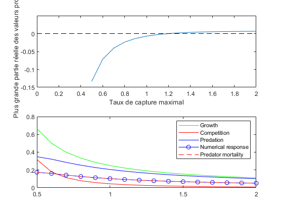
figure(4)
subplot(2,1,1)
aa=amin:da:amax;
plot(aa,Lambda,[0 amax],[0 0],'k--')
xlabel('Taux de capture maximal');ylabel('Plus grande partie réelle des valeurs propres')
ylim([-0.15 0.05]);
subplot(2,1,2)
Xe=Ue(:,1);Ye=Ue(:,2);
GROWTHeq=r*Xe;COMPETeq=Xe.^2./K;
PREDATIONeq=aa'.*Xe./(1+b*Xe).*Ye;NUMERICALRESPeq=e*aa'.*Xe./(1+b*Xe).*Ye;
MORTALITYeq=m*Ye;
plot(aa',GROWTHeq,'g',aa',COMPETeq,'r',aa',PREDATIONeq,'b',aa',NUMERICALRESPeq,'-ob',aa',MORTALITYeq,'--r')
legend('Growth','Competition','Predation','Numerical response','Predator mortality')
%subplot(2,2,3)
%plot(KK,abs(J11),KK,abs(J12),KK,abs(J21),KK,abs(J22))
%legend('J_{11}','J_{12}','J_{21}','J_{22}')
%subplot(2,2,4)
%plot(KK,abs(J11)./abs(J21),KK,ones(size(KK)))
a=atamp;
%plot(KK,YE,KK,YEnum(:,2),'or')

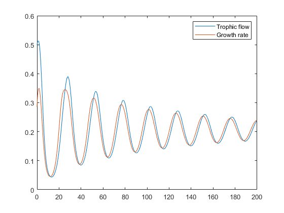
figure(5)
GROWTH=r*x.*(1-x/K00);
PREDATION=a*x./(1+b*x).*y;
plot(t,PREDATION,t,GROWTH)
legend('Trophic flow','Growth rate')

Equation solved.

fsolve completed because the vector of function values is near zero
as measured by the value of the function tolerance, and
the problem appears regular as measured by the gradient.


Equation solved.

fsolve completed because the vector of function values is near zero
as measured by the value of the function tolerance, and
the problem appears regular as measured by the gradient.


Equation solved.

fsolve completed because the vector of function values is near zero
as measured by the value of the function tolerance, and
the problem appears regular as measured by the gradient.


Equation solved.

fsolve completed because the vector of function values is near zero
as measured by the value of the function tolerance, and
the problem appears regular as measured by the gradient.


Equation solved.

fsolve completed because the vector of function values is near zero
as measured by the value of the function tolerance, and
the problem appears regular as measured by the gradient.


Equation solved.

fsolve completed because the vector of function values is near zero
as measured by the value of the function tolerance, and
the problem appears regular as measured by the gradient.


Equation solved.

fsolve completed because the vector of function values is near zero
as measured by the value of the function tolerance, and
the problem appears regular as measured by the gradient.


Equation solved.

fsolve completed because the vector of function values is near zero
as measured by the value of the function tolerance, and
the problem appears regular as measured by the gradient.


Equation solved.

fsolve completed because the vector of function values is near zero
as measured by the value of the function tolerance, and
the problem appears regular as measured by the gradient.


Equation solved.

fsolve completed because the vector of function values is near zero
as measured by the value of the function tolerance, and
the problem appears regular as measured by the gradient.


Equation solved.

fsolve completed because the vector of function values is near zero
as measured by the value of the function tolerance, and
the problem appears regular as measured by the gradient.


Equation solved.

fsolve completed because the vector of function values is near zero
as measured by the value of the function tolerance, and
the problem appears regular as measured by the gradient.


Equation solved.

fsolve completed because the vector of function values is near zero
as measured by the value of the function tolerance, and
the problem appears regular as measured by the gradient.


Equation solved.

fsolve completed because the vector of function values is near zero
as measured by the value of the function tolerance, and
the problem appears regular as measured by the gradient.


Equation solved.

fsolve completed because the vector of function values is near zero
as measured by the value of the function tolerance, and
the problem appears regular as measured by the gradient.


Equation solved.

fsolve completed because the vector of function values is near zero
as measured by the value of the function tolerance, and
the problem appears regular as measured by the gradient.


Equation solved.

fsolve completed because the vector of function values is near zero
as measured by the value of the function tolerance, and
the problem appears regular as measured by the gradient.


Equation solved.

fsolve completed because the vector of function values is near zero
as measured by the value of the function tolerance, and
the problem appears regular as measured by the gradient.


Equation solved.

fsolve completed because the vector of function values is near zero
as measured by the value of the function tolerance, and
the problem appears regular as measured by the gradient.


Equation solved.

fsolve completed because the vector of function values is near zero
as measured by the value of the function tolerance, and
the problem appears regular as measured by the gradient.


Equation solved.

fsolve completed because the vector of function values is near zero
as measured by the value of the function tolerance, and
the problem appears regular as measured by the gradient.


Equation solved.

fsolve completed because the vector of function values is near zero
as measured by the value of the function tolerance, and
the problem appears regular as measured by the gradient.


Equation solved.

fsolve completed because the vector of function values is near zero
as measured by the value of the function tolerance, and
the problem appears regular as measured by the gradient.


Equation solved.

fsolve completed because the vector of function values is near zero
as measured by the value of the function tolerance, and
the problem appears regular as measured by the gradient.


Equation solved.

fsolve completed because the vector of function values is near zero
as measured by the value of the function tolerance, and
the problem appears regular as measured by the gradient.


Equation solved.

fsolve completed because the vector of function values is near zero
as measured by the value of the function tolerance, and
the problem appears regular as measured by the gradient.


Equation solved.

fsolve completed because the vector of function values is near zero
as measured by the value of the function tolerance, and
the problem appears regular as measured by the gradient.


Equation solved.

fsolve completed because the vector of function values is near zero
as measured by the value of the function tolerance, and
the problem appears regular as measured by the gradient.

Published with MATLAB® R2019b